| Selathco 0.91 generated HTML | ||
| ( Table of contents ) | ||
1. Introduction
Before going deeply into details of the J-Sim system, a presentation of the theoretical background on which J-Sim and other similar tools are based should be given. This chapter is especially important for those who have never modelled any simulation of discrete processes, but can be useful for experienced users too, because it clarifies and explains all principles used in discrete simulations, and presents some recommendations how such a discrete-simulations modelling tool should work.
1.1. Fundamental Concepts of Discrete Simulation
As the word "discrete" says, discrete simulation is not executed continuously. Instead, it is divided into steps. Every simulation has its own time which will be called here simulation time. A simulation can be either finite or infinite. Wheter a simulation is finite or not cannot be determined easily because new steps can be created dynamically during execution of another step. Each step is executed at one exact point of simulation time. This time cannot be changed in any way during one simulation step. Two or even more steps can be executed at the same simulation time but it is not determined which of them will run first. Steps are never executed parallelly, but always sequentially. The time difference between two consequent simulation steps is usually a non-zero positive value. When one simulation step has finished and another one is being started, the simulation time must change - it jumps from the old value to the new. In fact, a simulation is just a passive object which does not do anything. But it can contain various number of processes which are active. The number of processes within a simulation can vary as time passes, existing processes can die, and thus disappear completely, and new processes can be created. Processes are active thanks to their pre-programmed life. Usually, processes do not share any common data but if there is such a need, it can be easily arranged. The thing which gives processes the possibility to be executed at several different time points is called reactivation points. A reactivation point is such a point in a process' life which separates parts to be executed during different simulation steps, and therefore at different times. This will be discussed in more detail in a following chapter.
However, the time differences between two consequent parts of a process' life does not necessarily correspond to the differences between two consequent simulation steps. The fact which breaks up this equality is that one simulation contains several processes, all of which have their corresponding life parts to be executed at different time points. Therefore, the simulation must always evaluate time at which the next step will be executed as the minimum value of all values requested by all processes within the simulation. The processes' life parts are interleaved - there can be number of simulation steps to be executed between two parts A and B of the same process. This number can be even unknown when the life part B is scheduled because another process run in the time interval between A and B can create thousands of life parts with differences between them so small that they will fit into the interval <A,B>.
To be able to work in the manner described above, every simulation has its own calendar where events are stored. An event is an object holding information about a required time point and a process that wants to be run at that time. All of the events are stored in the calendar in ascending order with regard to the time of events. When a new event is added to the calendar, it is inserted at a corresponding position, i.e. the time of previous event in the calendar is less than or equal to the new event's time, and the time of next event is greater than or equal to it.
An example on what it may look like is shown in the following figure:
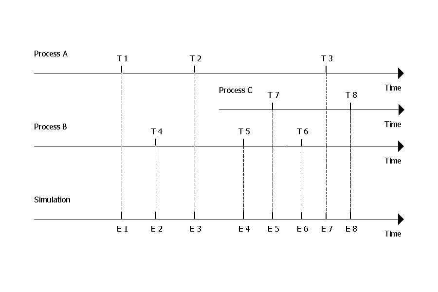
The Principle of Event Interleaving
Two processes (A and B) want to be executed; each of them has three events to be scheduled. Process A's events are scheduled at time points T1, T2 and T3, process B's events at time points T4, T5 and T6. Because T4 is greater than T1 but less than T2, it is put between these two events, and so on. Then, a new process, called C, is created and its' two events are inserted into the calendar. Although process A's and process B's events T3 and T5 (and perhaps T6) are already present in the calendar, process C's event T7 is inserted between them and its corresponding simulation step (a piece of process C's life) will be executed after T5 and before T6.
Note that none of the three processes knows anything about the two other processes' events. It does not even know that others may exist! It is a matter of the simulation to put all the required events in a good order and to select an appropriate process to run when it is demanded to execute a simulation step. Also note that eight simulation steps are needed to consume all the events depicted in the figure. But new events can be created during execution of the eight ones shown. This is the principle of infinite simulations. A simulation is infinite if it contains at least one infinite process. A process is infinite if it never reaches the end of its life, i.e. for every consumed event there is on average at least one new event created. The easiest way how to make a process infinite is to use a neverending loop which will contain a reactivation point in its body.
1.2. Simulation-Time to Real-Time Mapping
So far the simulation time and its property of discreteness has only been discussed. However, when a program is executed it is a continuous process of taking instructions and interpreting them. In J-Sim, there exists an exact way how to describe the relation between the simulation time and the real time. To better understand this subject, look at the scheme 1.2. on page 1.
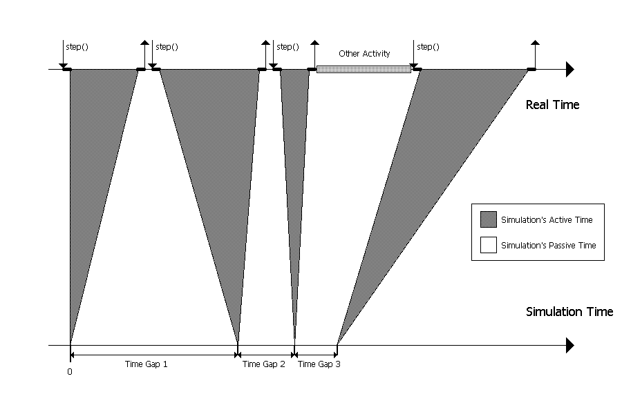
Simulation-Time to Real-Time Mapping
There are four events to be executed, each of them at a different time. Between them there are time gaps which can have any arbitrary length. The length can be zero, but that is a very special case discussed above - more simulation steps scheduled at the same time. The most important thing to be seen on the bottom axis is that every simulation step is zero time units long. That is a consequence of the fact that time cannot change during a simulation step.
At the upper axis which represents real time, a corresponding time interval for each of the four simulation steps can be found. They have a non-zero length, i.e. the execution of a step in real life is never infinitely short. Note that not all the time is spent by executing a process' code. There are little time intervals necessary for the system to switch between processes and there can be also time intervals that have nothing to do with the simulation at all. This interval is labeled as "Other Activity".
A simulation step begins when the user asks the simulation to execute a step. The simulation must select an appropriate process (1) and give it control. In that moment, the process gains full control over its life and nothing (neither the simulation nor other processes) can stop or interrupt it. It is fully in its own competence when the step will be finished. There are two ways how to finish a step. The process can either naturally die (i.e. its life terminates) or it can use a reactivation routine to establish a reactivation point. In the latter case, the process will be temporarily interrupted until another event belonging to this process is found in the calendar. Such an event can be added to the calendar either by the reactivation routine itself or by another process. In the former case, the process will not be able to run anymore.
1.3. Reactivation Points and Reactivation Routines
A reactivation point is such a point in a process' life where the process is temporarily interrupted (or suspended) until an event belonging to the process is found in the simulation's calendar. Every reactivation point terminates currently executed simulation step. As stated above, the currently running process has absolute power over simulation's real time. It can even deprive all other processes of the possibility to run by performing a neverending loop which does not contain any reactivation points. Once such a process is run and gets to this point, no other process will have a chance to run. Plus, the simulation step during which this process is run will never terminate and the programmer will therefore loose control over simulation's progress. Fortunately, such cases are completely useless in the domain of discrete simulations.
Every reactivation point is realized by a reactivation routine. In general, two kinds of reactivation points and their corresponding reactivation routines can be distinguished:
- A passivating routine terminates current simulation step and returns control to the simulation. It does not add any new event to the simulation's calendar. Therefore, the process which uses this routine will not be activated anymore unless other processes activate it. The process cannot be sure if and when it will be activated. The name of this routine is passivate.
- A temporarily passivating routine terminates current simulation step and returns control to the simulation, but in addition creates a new event belonging to this process and inserts it into the simulation's calendar. Therefore, the process can be sure that it will be activated in the future. This routine has one parameter determining the difference between current time and the time when the process has to be reactivated. The name of this routine is hold.
1.4. Scheduling Possibilities
In order to have a complete and more detailed overview of existing possibilities of scheduling, the following paragraphs will briefly characterize them.
First of all, every process should be activated to have a chance to run at all. The name of this operation is activate and it has one parameter determing the time of activation. A process can activate other processes at any time but the activation is usually done by the main program before the simulation starts. Once a process is activated and run it does not need another activation to run at another time, it can use the temporarily passivating routine.
Sometimes there is a need to cancel an already made scheduling and delete all events belonging to a process from the calendar. The name of this operation is cancel. As a result, the affected process will not run anymore unless it is newly activated. A process can cancel another process as well as itself.
The two remaining possibilities have been already mentioned above. It should be noted that the passivate operation does not alter the simulation's calendar in any way while the hold operation does. A process cannot passivate or temporarily passivate another process, only itself. Every attempt to passivate another process will result in an error.
1.5. Requirements for the Tool
Having the theoretical knowledge obtained in previous chapters, one can try to formulate some necessary requirements that the simulation tool should meet. These requirements concern the tool itself, but also the programming language in which the tool will be written:
- The programming language should be widely spread and well known to most developers (scientists).
- The programming language should be platform-independent in order to allow users to use the tool in all possible computing environments and to port user's simulations from one platform to another with minimum effort. Complete portability (source texts and runnable output) is preferrable to partial portability (source texts only, need to recompile in target environment).
- The programming language should offer a way how to create and run several processes concurrently, providing a safe method of their synchronization - temporary suspension followed by reactivation upon a received signal is necessary.
- The programming language should be object-oriented. This will allow the tool to provide basic classes that could be extended both in functionality and in data content by users.
- The tool should offer an easy way to create a simulation and a process. The preferrable way is the inheritance from already existing classes present in the tool.
- The tool should hide all implementation details and make process suspension and reactivation transparent for the user.
- The tool should provide two ways of running: in batch mode with output to the console, and in interactive mode with output to a graphics window. Therefore, graphics possibilities should be offered by the programming language and they should be preferrably platform-independent as well. In the latter case, the simulation should be driven by user's actions.
Now each requirement will be taken point-by-point to determine whether J-Sim meets it or not, and if it does, then in what way:
- J-Sim is written in 100%-pure Java. Today, Java is one of the most spread and well-known languages. Its runtime environments and compilers are available for free for most widely used platforms. Java is easy to learn and easy to use.
- Java pre-compiled code is interpreted in the target environment; therefore, both source texts and pre-compiled code are portable. In case of any problems, source texts provided with J-Sim can be used to generate new code, compiled in the target environment, thus 100-percent compatible with JVM (2) used.
- Java provides a class called Thread whose instances run parallelly with other such instances. Thread support is directly built into the language and therefore no additional library is necessary, like in the case of the C language. An efficient way of thread synchronization is provided directly in the language too. Every object has its own lock which can temporarily suspend currently running thread and reactivate it when a wake-up signal is received from another thread.
- Java is a fully object-oriented language, providing the concepts of classes, instances, encapsulation, inheritance and polymorphism (3) . Unlike in C++, the use of object principles is strictly mandatory in Java.
- J-Sim provides basic classes for simulation, process and queue. These classes can be either directly used or extended according to specific user's requirements.
- There are no special actions required in order to passivate or temporarily passivate a process. Two methods are provided in the process class whose use is very intuitive and easy. The user need not know any implementation details concerning suspension and reactivation.
- J-Sim provides two possibilities of running a simulation which can be dynamically switched. The first one is the batch mode, sending output to the console. The second one is the interactive mode, using a graphics window to control the simulation and to display simulation output. Both of them use only standard Java services and thus are fully portable. However, the possibilities of the target environment may limit their use (4) .
To avoid confusion at this point, it should be defined what exactly J-Sim is and what it is not. J-Sim is a tool which can help users to simulate behaviour of pseudo-parallel processes. J-Sim is not a complete, ready-to-run software, it always needs a user (programmer) who creates a simulation and processes and pre-programs them a meaningful sequence of actions called life.
- (1) It is a process which has an event at the top of simulation's calendar.
- (2) Java Virtual Machine
- (3) If you do not know what these terms mean, consult a textbook of object-oriented programming.
- (4) For example, older versions of MacOS do not have console output.
Converted by Selathco 0.91 on 01.09.2001 18:44 |